The hard non-linearities such as step functions are useful for modelling a categorical variable in neural networks. The gradient is zero everywhere for hard activations, which leads to difficulty in training using backpropagation. We review some technique proposed to estimate gradient such as straight through estimator.
Hard non-linearity
Hard non-linearities have gradient zero everywhere (e.g., step function). Following are two use cases for using hard activation functions:
- Categorial Variable
Hard non-linearities are useful in modelling choices we encounter in our everyday life. Consider a generative neural network which can generate images for digit 1 up to 10 on request. It’s challenging to backpropagate through the categorical variable.
- Conditional computation or Sparse Representation
Usecase I am exploring is to prevent backpropagation from updating certain parts of a network to avoid catastrophic forgetting of tasks learned previously. It’s similar to conditional computation task proposed by Bengio [1].
Stocastic Binary Neuron
Stochastic binary neurons are thresholding function on the input value (a_i). $$ h_i = f(a_i, z_i) = 1_{z_i > sigmoid(a_i)} $$
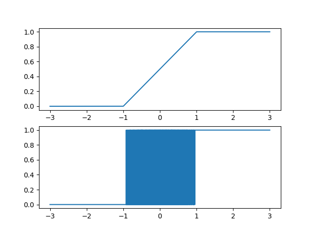
Here $z_i$ is sampled using Bernoulli for stocastic neuron. Figure below shows how the output of stocastic binary neuron looks like on whole input range of sigmoid. Between the active range of [-1,1] output is stocastic in nature.

Below is the code for Stocastic Binary Neuron (Courtesy [3]: https://github.com/Wizaron/binary-stochastic-neurons/blob/master/utils.py)
class Hardsigmoid(nn.Module):

    def __init__(self):
        super(Hardsigmoid, self).__init__()
        self.act = nn.Hardtanh()

    def forward(self, x):
        return (self.act(x) + 1.0) / 2.0

class BernoulliFunctionST(Function):

    @staticmethod
    def forward(ctx, input):
        return torch.bernoulli(input)

    @staticmethod
    def backward(ctx, grad_output):
        return grad_output

BernoulliST = BernoulliFunctionST.apply
Getting the Above figure:
import torch
from matplotlib import pyplt

hard_sigmoid = HardSigmoid()
x = torch.linspace(-3,3,10000)
y = hard_sigmoid(x)
y2 = BernoulliFunctionST(y)
pyplt.subplot(2,1,1)
pyplt.plot(x,y)
pyplt.subplot(2,1,2)
pyplt.plot(x,y2)
Approaches for gradient estimation through hard non-linearities
Gradient can be estimated following four approaches compared by Bengio [1]:
Unbiased Gradient Estimator
Bengio [1] proposed an unbiased gradient estimator and a centered estimator which was shown to have minimum variance.
$$ g_i = (h_i - sigm(a)).Loss $$
We can use this unbiased gradient estimator above for backpropogation which gives us ability to switch off part of network.
Decompose Binary stocastic neuron
Stocastic additive or multiplicative noise
Straight through Estimator
Straight through Estimators just copy the gradient through non-linearity. Stocastic binary neuron would directly use gradient at output (h_i) at input (a_i).
$$ \frac{\partial L}{\partial a_i} = \frac{\partial L}{\partial h_i} * \partial sigmoid $$
They found it’s better to multiply gradient with derivative of sigmoid while copying the gradient.
Questions
References
- [1] Bengio, Yoshua, Nicholas Léonard, and Aaron Courville. “Estimating or propagating gradients through stochastic neurons for conditional computation.” arXiv preprint arXiv:1308.3432 (2013).
- [ 2] Jang, Eric, Shixiang Gu, and Ben Poole. “Categorical reparameterization with gumbel-softmax.” arXiv preprint arXiv:1611.01144 (2016).
- [3] Pytorch Implementation for stocastic Neuron taken from github @Wizaron
- [4] r2rtt.com blog by Silviu Pitis
Future Work
Include Gumble softmax trick here.